7  Property Sales

It is worthwhile to study trends in property sales and the variables that affect this as everybody needs somewhere affordable to live.

This lesson examines property sales in North Shore city, using data recorded each December between 1999 and 2007. There are a total of 3788 properties, with about 420 being sold per December. This data was supplied by the Real Estate institute of New Zealand, with analysis conducted by Neil Binnie (Auckland University of Technology).

Data

Data Summary

3788 observations

12 variables

Variable	Type	Information
Year	Continuous
Zone	Categorical
Suburb	Categorical
List Price	Continuous	NZD ($).
Selling Price	Continuous	NZD ($).
Sell date	Continuous/Date	YYYY-MM-DD
List date	Continuous
Days to sell	Continuous
Number of bedrooms	Categorical or Discrete
Type	Categorical	7 levels: APT (Apartment), H & I (Home and Income), R (Residential), RIB (Residential Investment Block), RS (Residential Section), TH (Town House), U (Unit).
Land area m2	Continuous	Metres squared.
GV	Continuous	Government valuation of property NZD ($).

There is 1 file associated with this presentation. It contains the data you will need to complete the lesson tasks.

Download North Shore 99-07 December.xls

Video

Objectives

Learning Objectives

New skills and concepts:

1. Data wrangling - cleaning, subsetting, new variables.

2. Bar plots, single and multiple.

Reinforcing skills and concepts seen in earlier lessons:

1. Read and format data.

2. Summarise variables.

3. Box plots.

4. Histograms.

Tasks

0. Read and Format data

0a. Read in the data

Task

First check you have installed the package readxl (see Section 2.6) and set the working directory (see Section 2.1), using instructions in Getting started with R.

Load the data into R.

Important Information

Name your data property for easier reference later.

Previous Lesson

To load the data in R we run code analogous to Task 0 in Cockles Section 3.0.1

Code

The code has been hidden initially, so you can try to load the data yourself first before checking the solutions.

Code

#loads readxl package
library(readxl) 

#loads the data file and names it property
property<-read_xls("North Shore 99-07 December.xls")

#view beginning of data frame
head(property) 

Solution

Code

#loads readxl package
library(readxl) 

Warning: package 'readxl' was built under R version 4.2.2

Code

#loads the data file and names it property
property<-read_xls("North Shore 99-07 December.xls")

#view beginning of data frame
head(property) 

# A tibble: 6 × 12
   Year  Zone Suburb List …¹ Selli…² `Sell date`         List …³ Days …⁴ Numbe…⁵
  <dbl> <dbl> <chr>  <chr>     <dbl> <dttm>              <chr>   <chr>   <chr>  
1  1999     7 Takap… 525000   525000 1999-05-24 00:00:00 36294   10      0      
2  1999     7 Takap… 530000   530000 1999-08-20 00:00:00 36294   98      0      
3  1999     7 Takap… 565000   565000 1999-06-03 00:00:00 36294   20      0      
4  1999     6 Birke… 135000   120000 1999-11-24 00:00:00 36445   43      1      
5  1999     3 Albany 159000   159000 1999-11-19 00:00:00 36434   49      2      
6  1999     4 Brown… 149000   135000 1999-12-20 00:00:00 36448   66      2      
# … with 3 more variables: Type <chr>, `Land Area m2` <chr>, GV <chr>, and
#   abbreviated variable names ¹​`List Price`, ²​`Selling Price ($)`,
#   ³​`List Date`, ⁴​`Days to Sell`, ⁵​`Number of Bedrooms`
# ℹ Use `colnames()` to see all variable names

Most of the variables in this data frame are self explanatory, although there are 2 exceptions. Type is a factor variable indicating the type of property, with levels APT= Apartment, H & I = Home and Income, R = Residential, RIB= Residential Investment Block, RS = Residential Section, TH = Town House, and U = Unit. GV is the government valuation of the property for rating purposes, this is sometimes used as an approximation of property worth.

0b. Format the data

Task

Recode List Price, Days to Sell, Number of Bedrooms, Land Area m2 and GV as numeric variables.

Important Information

It is ok to ignore the warning \(\verb!Warning: NAs introduced by coercion!\), this is what we want to happen with the * values in the data. Note that \(\verb!warnings!\) still allow code to be executed (although they advise something unexpected may be happening), while \(\verb!errors!\) will prevent code from running.

Note that when we refer to variables with spaces in their names we must enclose them in backticks. If you wish to avoid this, you can rename the variables to remove spaces, as we have done in previous lessons e.g Cockles Task 0. Section 3.0.1.

Code

Code

property$`List Price`<-as.numeric(property$`List Price`)
property$`Days to Sell`<-as.numeric(property$`Days to Sell`)
property$`Number of Bedrooms`<-as.numeric(property$`Number of Bedrooms`)
property$`Land Area m2`<-as.numeric(property$`Land Area m2`)
property$GV<-as.numeric(property$GV)

Solution

Code

property$`List Price`<-as.numeric(property$`List Price`)

Warning: NAs introduced by coercion

Code

property$`Days to Sell`<-as.numeric(property$`Days to Sell`)

Warning: NAs introduced by coercion

Code

property$`Number of Bedrooms`<-as.numeric(property$`Number of Bedrooms`)

Warning: NAs introduced by coercion

Code

property$`Land Area m2`<-as.numeric(property$`Land Area m2`)

Warning: NAs introduced by coercion

Code

property$GV<-as.numeric(property$GV)

Warning: NAs introduced by coercion

1. Summary Statistics, Histogram, Clean data

1a. Summary Statistics

Task

First calculate some descriptive statistics (number of observations, mean, quartiles, maximum) for various continuous variables in the data set above, in order to see if there are any interesting features or obvious strange values. This can be achieved using the apply() function.

The variables of interest are Selling Price ($) (column 5), Days to Sell (column 8), Number of Bedrooms (column 9), Land Area m2 (column 11), and GV (column 12).

Code

We use MARGIN=2 to indicate we want summaries for each column (MARGIN=1 summarises by rows).

FUN= specifies the function we wish calculate for each column. Note when FUN=quantile there is an additional argument probs= to give the quantile level. Sometimes it is necessary to include na.rm=T to avoid errors from missing data.

Code

#number of observations
apply(property[,c(5,8,9,11,12)],MARGIN=2,FUN=length)  

#minimum
apply(property[,c(5,8,9,11,12)],MARGIN=2,FUN=min,na.rm=T)  

#mean
apply(property[,c(5,8,9,11,12)],MARGIN=2,FUN=mean,na.rm=T) 

#lower quartile
apply(property[,c(5,8,9,11,12)],MARGIN=2,FUN=quantile,probs=0.25,na.rm=T)

#middle quartile/median
apply(property[,c(5,8,9,11,12)],MARGIN=2,FUN=quantile,probs=0.5,na.rm=T) 

Also calculate the upper quartile and the mean for the variables of interest.

Solution

Code

#number of observations
apply(property[,c(5,8,9,11,12)],MARGIN=2,FUN=length) 

 Selling Price ($)       Days to Sell Number of Bedrooms       Land Area m2 
              3788               3788               3788               3788 
                GV 
              3788 

Code

#minimum
apply(property[,c(5,8,9,11,12)],MARGIN=2,FUN=min,na.rm=T)  

 Selling Price ($)       Days to Sell Number of Bedrooms       Land Area m2 
             59000                  0                  0                  0 
                GV 
                 0 

Code

#mean
apply(property[,c(5,8,9,11,12)],MARGIN=2,FUN=mean,na.rm=T) 

 Selling Price ($)       Days to Sell Number of Bedrooms       Land Area m2 
      434772.86510           56.48828            3.19017         2945.26554 
                GV 
      319314.25759 

Code

#lower quartile
apply(property[,c(5,8,9,11,12)],MARGIN=2,FUN=quantile,probs=0.25,na.rm=T)

 Selling Price ($)       Days to Sell Number of Bedrooms       Land Area m2 
            260000                 15                  3                533 
                GV 
            197000 

Code

#middle quartile/median
apply(property[,c(5,8,9,11,12)],MARGIN=2,FUN=quantile,probs=0.5,na.rm=T) 

 Selling Price ($)       Days to Sell Number of Bedrooms       Land Area m2 
            361000                 31                  3                685 
                GV 
            280000 

Code

#upper quartile
apply(property[,c(5,8,9,11,12)],MARGIN=2,FUN=quantile,probs=0.75,na.rm=T) 

 Selling Price ($)       Days to Sell Number of Bedrooms       Land Area m2 
          515000.0               60.0                4.0              900.5 
                GV 
          400000.0 

Code

#maximum
apply(property[,c(5,8,9,11,12)],MARGIN=2,FUN=max,na.rm=T)

 Selling Price ($)       Days to Sell Number of Bedrooms       Land Area m2 
           8300000               1552                 16            4000000 
                GV 
           3500000 

There appear to be some unrealistic minimum values for certain variables e.g. 0 Days to Sell and Land Area of 0 metres squared.

Based on the difference between the upper quartiles (values 75% of the data is less than) and the maximums, some variables are also highly skewed e.g. Selling Price ($515,000 upper quartile and $8,300,000 maximum), Number of Bedrooms (4 and 16), Land Area (900.5 m2 and 4,000,000 m2).

1b. Histogram

Task

These features can also be examined visually using histograms. Draw a histogram of Selling Price ($).

Important Information

Implement a maximum x axis value of 1.5 million to avoid a highly skewed graph. This idea is discussed in detail in the video for this lesson, and you could remove this xlim=c() restriction from the code to see the difference.

Code

As well as indicating col= using numbers or factor variables, we can provide specific colour names. The histogram below shows an example of this, you can google R colour palette to see more built-in colour options.

Code

hist(property$`Selling Price ($)`,xlab="Selling Price ($)", main="North Shore Selling Prices", col="plum2",xlim=c(0,1500000),breaks=50)

Consider what we could change in the code below to show more detail in the histogram.

Solution

Code

#less breaks, less detail
hist(property$`Selling Price ($)`,xlab="Selling Price ($)", main="North Shore Selling Prices", col="plum2",xlim=c(0,1500000),breaks=50)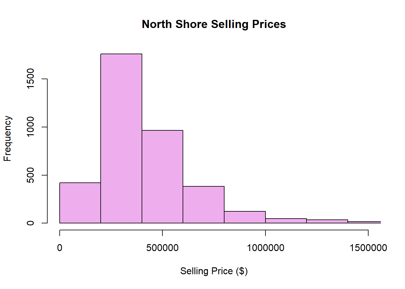

Code

#more breaks, more detail
hist(property$`Selling Price ($)`,xlab="Selling Price ($)", main="North Shore Selling Prices", col="plum2",xlim=c(0,1500000),breaks=100)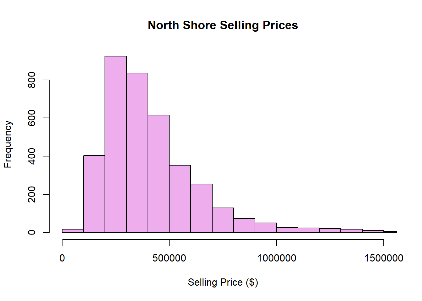

The distribution of North shore selling prices is unimodal with a peak of approximately $250,000. It is right skewed (even after excluding extreme values).

1c. Cleaning the data

Task

As we have seen in the video, there are some problems with this data. For example, some residential properties (Type = R) have no bedroom (i.e. Number of Bedrooms = 0) !

Since a residential house without any bedroom does not make sense, it is most likely that the number of bedrooms in these properties is simply missing (e.g. unknown or not recorded) rather than 0.

Correct the data of these mistaken properties by changing the value in the Number of Bedrooms column from 0 to NA (as NA denotes a missing value).

Code

Open the property data frame in a new tab by running the code below.

Code

View(property)

Click the Filter button, then in the box at the top of the Type column type “R” to filter residential properties. We can see there are 3 properties of Type = R that have no bedrooms. We will replace these 0s with NAs.

Code

#finding the rows of property corresponding to Type=R with 0 bedrooms, then indicating the Number of Bedrooms column (column 9). 
#Overwriting these entries with NA

property[which(property$`Number of Bedrooms`=="0"&property$Type=="R"),9]<-NA

Check the data frame again using the Filter procedure above, the first 3 entries of Number of Bedrooms when Type=R should now be NA.

Repeat this for the other mistaken property values mentioned in the video.

Solution

Open the property data frame in a new tab by running the code below.

Code

View(property)

Click the Filter button, then in the box at the top of the Type column type “R” to filter residential properties. We can see there are 3 properties of Type = R that have no bedrooms. We will replace these 0s with NAs.

Code

#finding the rows of property corresponding to Type=R with 0 bedrooms, then indicating the Number of Bedrooms column (column 9). 
#Overwriting these entries with NA

property[which(property$`Number of Bedrooms`=="0"&property$Type=="R"),9]<-NA

Check the data frame again using the Filter procedure above, the first 3 entries of Number of Bedrooms when Type=R should now be NA.

2. Summary Tables, Bar Plots

2a. Summary Tables

Task

Investigate the way the North Shore property market has been performing between 1999 and 2007, by examining changes in Number of Sales, the median Number of Days to Sell a property, and the median Selling Price ($) per December month.

This can be carried out using the function tapply().

Code

Getting the length of Selling Price ($) for each Year is a proxy for the number of sales that year.

Code

tapply(property$`Selling Price ($)`,INDEX=property$Year,FUN=length)

It is a similar process to find the median Days to Sell by December month. There are some NAs in the Days to Sell column, so we want to remove these when calculating the median.

Code

tapply(property$`Days to Sell`,INDEX=property$Year,FUN=median,na.rm=T)

Finally, modify code above to calculate the median Selling Price($) by December month.

Solution

Getting the length of Selling Price ($) for each Year is a proxy for the number of sales that year.

Code

tapply(property$`Selling Price ($)`,INDEX=property$Year,FUN=length)

1999 2000 2001 2002 2003 2004 2005 2006 2007 
 306  275  418  485  604  504  386  522  288 

It is a similar process to find the median Days to Sell by December month. There are some NAs in the Days to Sell column, so we want to remove these when calculating the median.

Code

tapply(property$`Days to Sell`,INDEX=property$Year,FUN=median,na.rm=T)

1999 2000 2001 2002 2003 2004 2005 2006 2007 
  46   65   48   25   22   27   29   30   35 

Calculate the median Selling Price($) by December month.

Code

tapply(property$`Selling Price ($)`,INDEX=property$Year,FUN=median,na.rm=T)

  1999   2000   2001   2002   2003   2004   2005   2006   2007 
240500 257000 260000 287500 349500 400000 445000 490000 513750 

There does not appear to be a pattern in the number of property sales per year or the number of days to sell, aside from some correspondence between less days to sell and a greater number of sales (equally, more days to sell and a smaller number of sales).

There is a clear upward trend in median selling price by year.

2b. Bar Plot

Task

We can create bar plots of these statistics for easier interpretation.

Code

For the Number of Sales per December month we assign the tapply() command we used earlier to an object called salesTable, then can create a bar plot using the function barplot() on this.

Code

salesTable<-tapply(property$`Selling Price ($)`,INDEX=property$Year,FUN=length)

barplot(salesTable,xlab="Year",ylab="Number of Sales",main="December Property Sales on North Shore by Year")

Generate bar plots for median Days to Sell and median Selling Price ($) per December month.

Solution

Code

#Number of sales
salesTable<-tapply(property$`Selling Price ($)`,INDEX=property$Year,FUN=length)

barplot(salesTable,xlab="Year",ylab="Number of Sales",main="December Property Sales on North Shore by Year")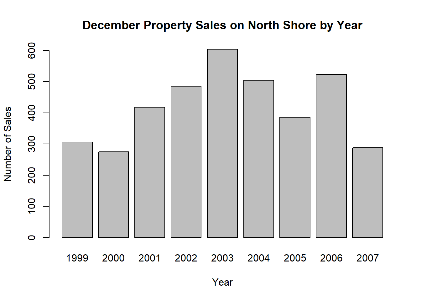

Code

#Median days to sell
salesTable2<-tapply(property$`Days to Sell`,INDEX=property$Year,FUN=median,na.rm=TRUE)

barplot(salesTable2,xlab="Year",ylab="Days to Sell",main="Median December Days to Sell on North Shore by Year")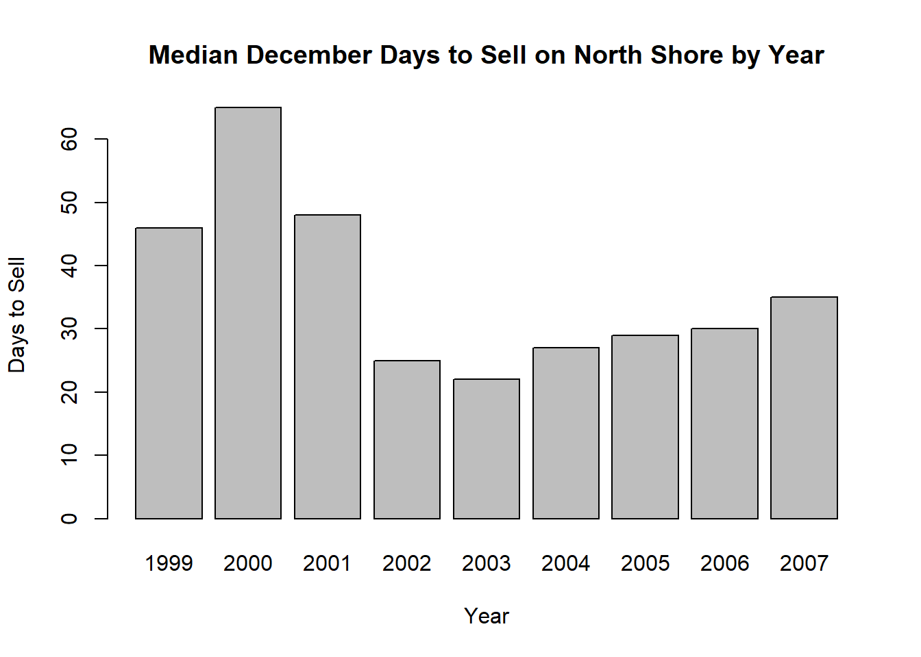

Code

#Median selling price
salesTable3<-tapply(property$`Selling Price ($)`,INDEX=property$Year,FUN=median,na.rm=TRUE)

barplot(salesTable3,xlab="Year",ylab="Selling Price ($)",main="Median December Selling Price on North Shore by Year")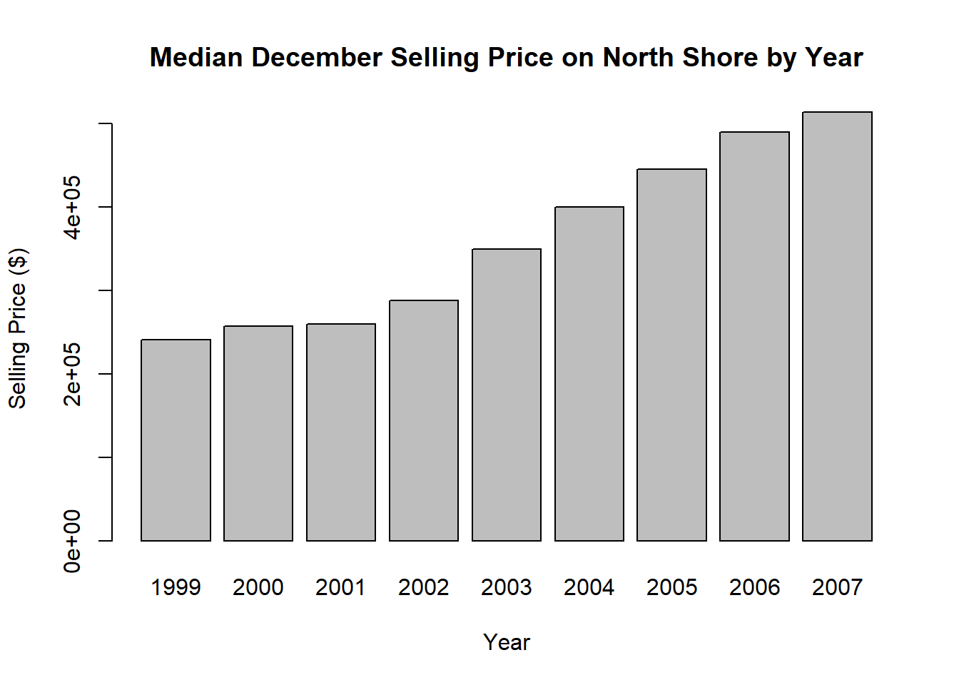

These bar plots make it easier to identify the patterns previously discussed. We can also see that the median days to sell dropped quite dramatically from 2001 to 2002, and has been slowly increasing since then.

2c. Multiple Bar Plots

Task

Construct a table showing the relationship between Number of Bedrooms and Type of property, this can be achieved using the table() function.

Using this table, draw a stacked bar graph to investigate the Number of Bedrooms each Type of properties has.

Code

Code

#dnn= can be provided a vector of the variable names, so it displays these on the table
table(property$`Number of Bedrooms`,property$Type,dnn=c("Number of Bedrooms","Type")) 

Code

#convert table above (without variable names) into a matrix to supply heights to bars
propertyMatrix<-as.matrix(table(property$`Number of Bedrooms`,property$Type)) 

#barplot, with bars corresponding to the same type of property stacked on top of each other (beside=FALSE). 
#The other arguments work in the same way as they have been used for previous plots e.g labelling axes, giving colour for different bars.
barplot(propertyMatrix,beside=FALSE,names=c("APT","H & I","R","RIB","RS","TH","U"),col=1:14,
 ylab="Count",xlab="Type",main="Number of Bedrooms by Type of Property")

#legend
#since our bar plot has filled bars rather than points, we can display squares of colour on our legend using fill= instead of col=
legend("topright",legend=levels(as.factor(property$`Number of Bedrooms`)),fill= 1:14)

We can get a better view of the plot by clicking the Show in New Window button in the top right corner.

Solution

Code

#dnn= can be provided a vector of the variable names, so it displays these on the table
table(property$`Number of Bedrooms`,property$Type,dnn=c("Number of Bedrooms","Type")) 

                  Type
Number of Bedrooms  APT  H&I    R  RIB   RS   TH    U
                0     3    1    0    0   29    0    1
                1    54    0    7    0    0    4    9
                2   118    0  143    2    1   83  200
                3    50    8 1157    2    2  346   80
                4     5   21  722    1    0   93   12
                5     0   10  188    0    0    4    2
                6     0    5   35    1    0    2    2
                7     0    2    7    0    0    0    0
                8     0    0    2    0    0    0    0
                16    0    0    0    1    0    0    0

Code

#convert table above (without variable names) into a matrix to supply heights to bars
propertyMatrix<-as.matrix(table(property$`Number of Bedrooms`,property$Type)) 

#barplot, with bars corresponding to the same type of property stacked on top of each other (beside=FALSE). 
#The other arguments work in the same way as they have been used for previous plots e.g labelling axes, giving colour for different bars.
barplot(propertyMatrix,beside=FALSE,names=c("APT","H & I","R","RIB","RS","TH","U"),col=1:14,
 ylab="Count",xlab="Type",main="Number of Bedrooms by Type of Property")

#legend
#since our bar plot has filled bars rather than points, we can display squares of colour on our legend using fill= instead of col=
legend("topright",legend=levels(as.factor(property$`Number of Bedrooms`)),fill= 1:14)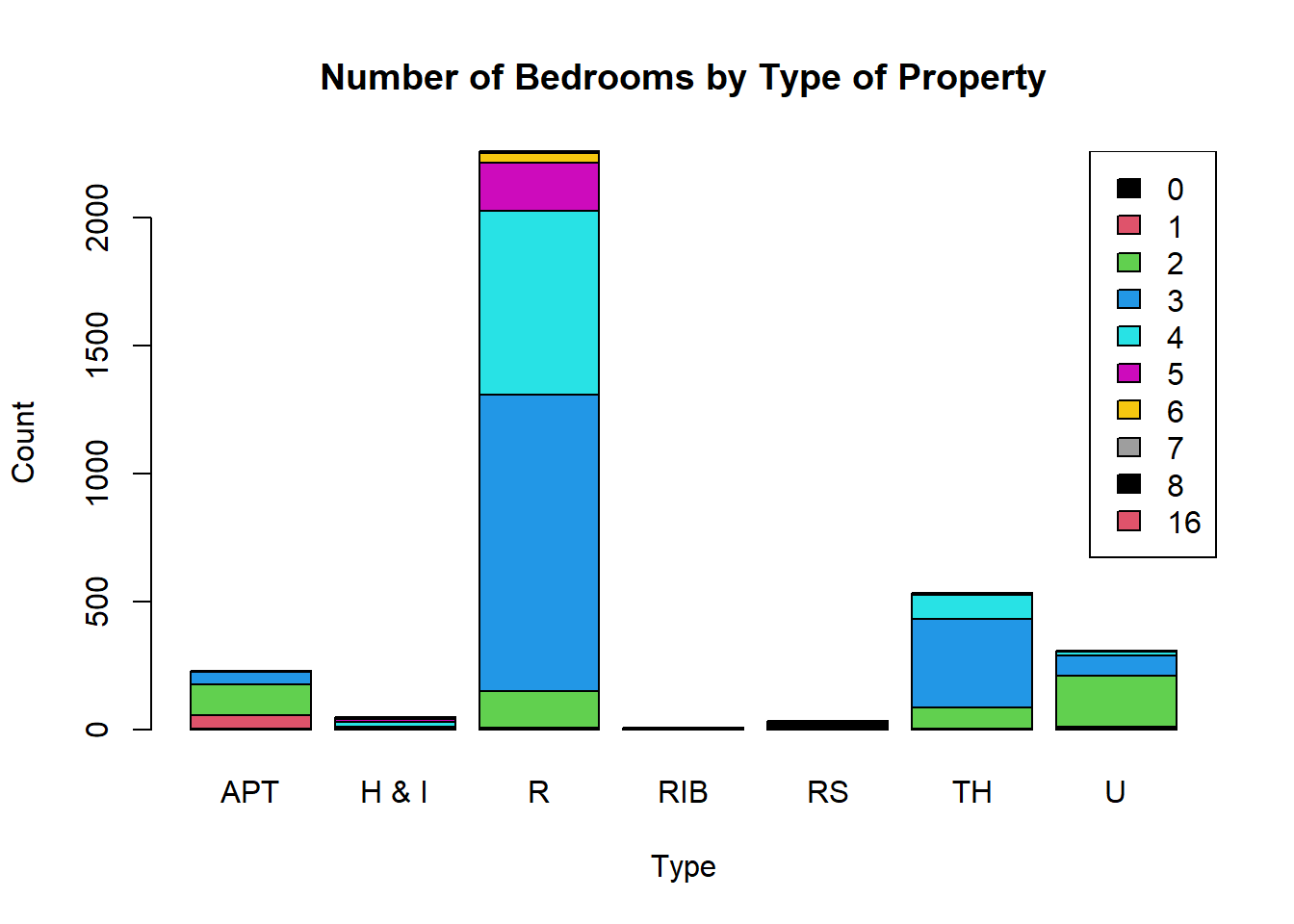

We can get a better view of the plot by clicking the Show in New Window button in the top right corner.

Apartments have a fairly even split between 1, 2 and 3 bedrooms. 3 or 4 bedrooms are most common for residential properties, with a good proportion of 5 bedroom properties too. All residential sections have no bedrooms (as they are purchased without houses). Units tend to be slightly larger than apartments, having 2 or 3 bedrooms, and town houses are a bit larger than these with 2-4 bedrooms.

3. Box Plots

3a. Box Plot (response by predictor)

Task

Investigate the changes in the median Selling Price ($) of the North Shore properties between Years 1999 and 2007 using box plots.

Important Information

Your initial box plot may look a bit strange, adding horizontal=T will rotate it and make it easier to see the distributions.

Previous Lesson

Have a look at the code in Dolphins Task 2b. Section 5.0.3 to generate this box plot.

Code

Code

boxplot(property$`Selling Price ($)`~property$Year,horizontal=T, main="Selling Price of North Shore Properties by Year")

Solution

Code

boxplot(property$`Selling Price ($)`~property$Year,horizontal=T, main="Selling Price of North Shore Properties by Year")

Previous Lesson

See Task 1a. (Section 3.0.2) in Cockles for interpretation of box plots.

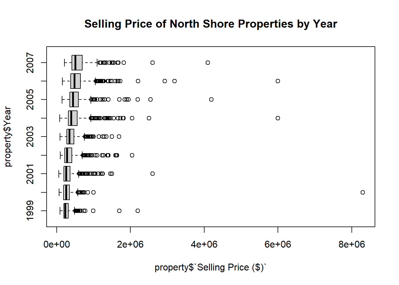
3b. Box Plots (subsetting)

Task

Draw a box plot of Selling Price ($) grouped by Suburb.

Since there are 49 different suburbs in this data, we cannot include all of them at once if we want an interpretable graph. You can try this by modifying the code, and will see the box plots are too small and squished to give us any useful information.

Instead, first create a subset of the data frame containing only data that corresponds to the Suburbs - Albany OR Devonport OR Glenfield OR Northcote OR Takapuna. Then construct a box plot using this data.

Previous Task

Following subsetting, the box plot can be constructed by modifying code from Task 3a.

Code

Code

property2<-property[which(property$Suburb=="Albany"|property$Suburb=="Devonport"|property$Suburb=="Glenfield"|property$Suburb=="Northcote"|property$Suburb=="Takapuna"),]

Code

boxplot(property2$`Selling Price ($)`~property2$Suburb,horizontal=T, main="Selling Price of North Shore Properties by Suburb")

Solution

Code

property2<-property[which(property$Suburb=="Albany"|property$Suburb=="Devonport"|property$Suburb=="Glenfield"|property$Suburb=="Northcote"|property$Suburb=="Takapuna"),]

Code

boxplot(property2$`Selling Price ($)`~property2$Suburb,horizontal=T, main="Selling Price of North Shore Properties by Suburb")

Previous Lesson

See Task 1a. (Section 3.0.2) in Cockles for interpretation of box plots.

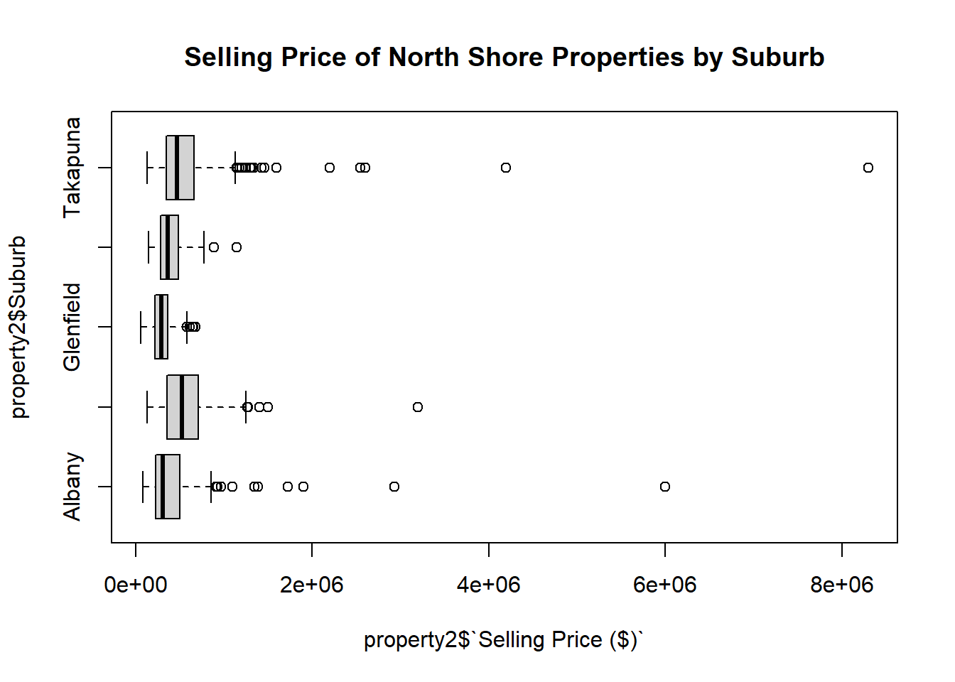
3c. Box Plots (subsetting)

Task

Draw a box plot of Selling Price ($) grouped by Number of Bedrooms.

Since the data contains only one property with 16 bedrooms, first create a subset of the data which removes this property.

Code

Code

#subsets data frame to only include rows where properties do not have 16 bedrooms
property3<-property[which(property$`Number of Bedrooms`!="16"),] 

Try to create the box plot first, then reveal the code below.

Code

boxplot(property3$`Selling Price ($)`~property3$`Number of Bedrooms`,horizontal=T, main="Selling Price of North Shore Properties by No. of Bedrooms")

Solution

Code

#subsets data frame to only include rows where properties do not have 16 bedrooms
property3<-property[which(property$`Number of Bedrooms`!="16"),] 

Try to create the box plot first, then reveal the code below.

Code

boxplot(property3$`Selling Price ($)`~property3$`Number of Bedrooms`,horizontal=T, main="Selling Price of North Shore Properties by No. of Bedrooms")

Previous Lesson

See Task 1a. (Section 3.0.2) in Cockles for interpretation of box plots.

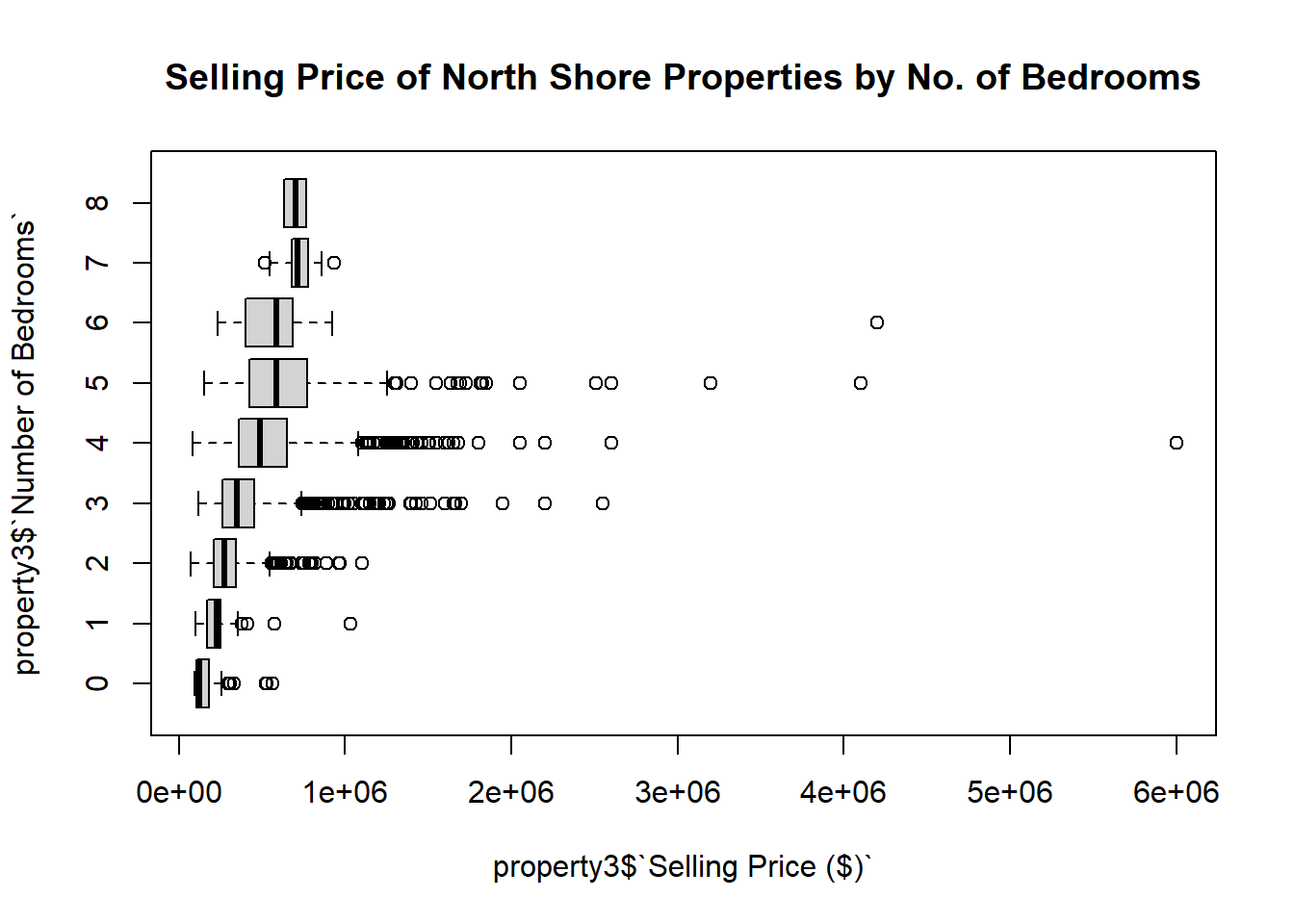
4. New Variables, Histograms

Task

Investigate how the List Price compares to the Selling Price ($) for the North Shore properties sold between 1999 and 2007 by drawing a histogram.

We want to only include rows where values of List Price are not equal to 0, as when List Price=0 this is equivalent to the data being missing. From these values, calculate a new variable Diff Price that is equal to the difference between List Price and the Selling Price ($) and plot a histogram of this.

Previous Task

You can modify the code from Task 3c. to exclude List Price values that are equal to 0.

Code

Include only List Price values not equal to 0.

Code

property4<-property[which(property$`List Price`!=0),]

Calculate new variable of the difference between List Price and Selling Price.

Code

property4$`Diff Price`<-property4$`List Price`- property4$`Selling Price ($)`

Create a histogram, complete with labels and an appropriate number of breaks, for Diff Price.

Code

hist(property4$`Diff Price`,xlab="Difference ($)", main="Difference between List Price and Selling Price of North Shore Properties",breaks=50)

Exclude the few very large positive and negative difference to get a better picture of the distribution of most values.

Code

#new data frame which only includes properties where the difference between list and selling price lies between -60000 and 200000
property5<-property4[which(-60000<=property4$`Diff Price`&property4$`Diff Price`<=200000),]

#we have excluded 12 properties
nrow(property4)
nrow(property5)  

Create a second histogram, complete with labels and an appropriate number of breaks, for Diff Price in this reduced data frame.

Code

hist(property5$`Diff Price`,xlab="Difference ($)", main="Difference between List Price and Selling Price \n of North Shore Properties",breaks=50)

Solution

Code

property4<-property[which(property$`List Price`!=0),]

Code

property4$`Diff Price`<-property4$`List Price`- property4$`Selling Price ($)`

Code

hist(property4$`Diff Price`,xlab="Difference ($)", main="Difference between List Price and Selling Price of North Shore Properties",breaks=50)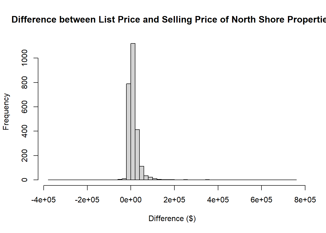

Code

#new data frame which only includes properties where the difference between list and selling price lies between -60000 and 200000
property5<-property4[which(-60000<=property4$`Diff Price`&property4$`Diff Price`<=200000),]

#we have excluded 12 properties
nrow(property4)

[1] 2540

Code

nrow(property5)  

[1] 2528

Code

hist(property5$`Diff Price`,xlab="Difference ($)", main="Difference between List Price and Selling Price \n of North Shore Properties",breaks=50)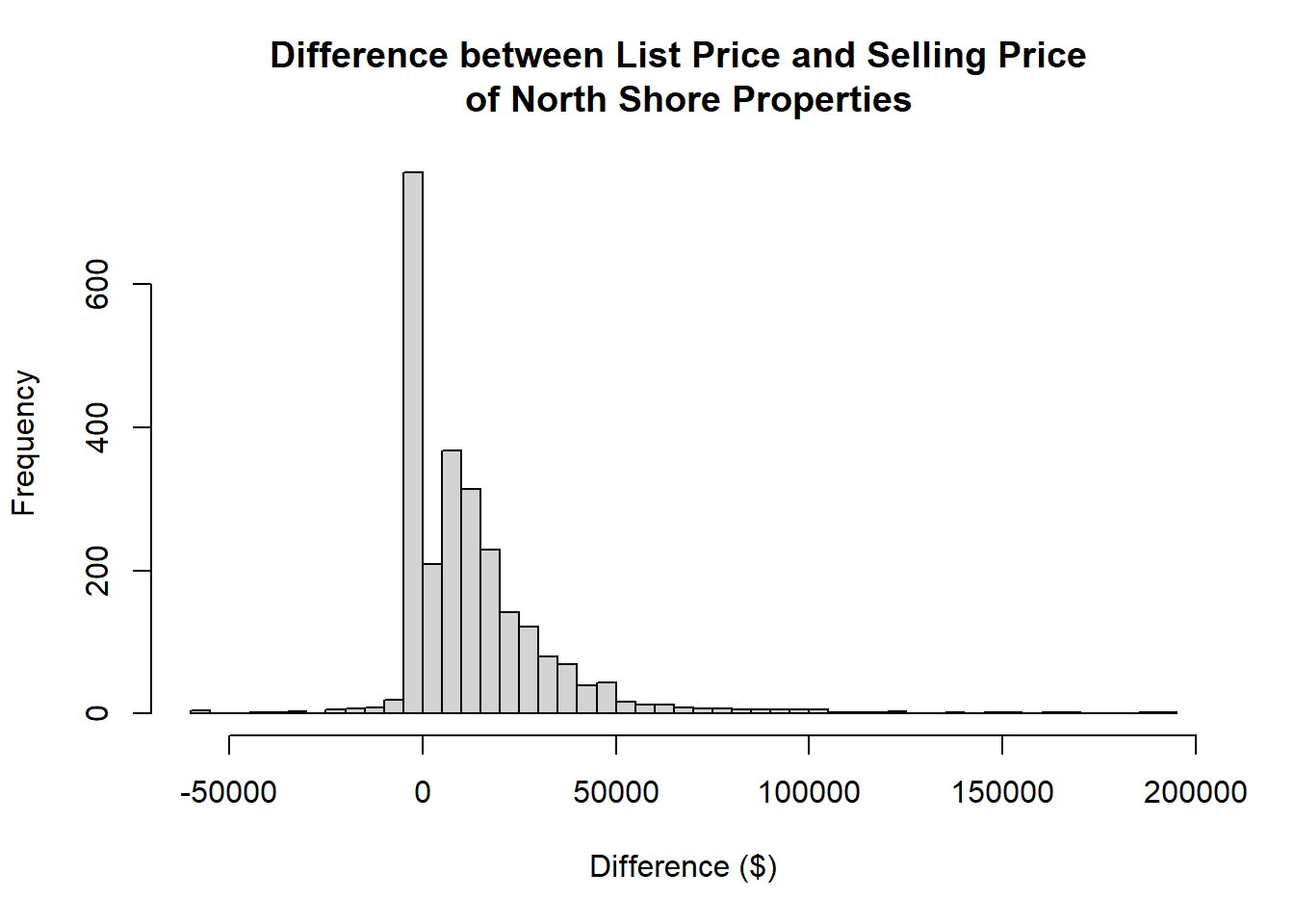

Previous Task

See Task 1b. for an example of histogram interpretation

5. New Variables, Box Plots

Task

Investigate how the Selling Price ($) compares to the Government Valuation (GV) for the North Shore properties sold between 1999 and 2007, using box plots.

Exclude values where GV is equal to 0, as this is equivalent to the data being missing.

There are also two other properties whose GV values are mistaken as 1050 and 430, instead of 1050000 and 430000 respectively. Hence, correct these values.

Calculate the difference between the Selling Price ($) and the GV to make a new variable GV Diff Price.

Finally, draw a box plot of the difference between Selling Price ($) and GV.

Previous Task

See Task 4 for the exclusion of values equal to 0, and creation of new variables.

See Task 1d. for the overwriting of incorrect values.

See Task 3 for box plot construction.

Code

Include only values where GV is not equal to 0.

Code

#subsetting property to include only GV values that are not equal to 0
property6<-property[which(property$GV!=0),]

Correct erroneous values.

Code

#finding the row of property corresponding to GV=430, then indicating the GV column (column 12). 
#Overwriting this entry with 430000
property6[which(property6$GV=="430"),12]<-430000 
property6[which(property6$GV=="1050"),12]<-1050000

Calculate the difference between the Selling Price ($) and the GV.

Code

#calculating the difference
property6$`GV Diff Price`<- property6$`Selling Price ($)`-property6$GV 

Box plot of this difference variable by year.

Code

boxplot(property6$`GV Diff Price`~property6$Year,horizontal=T, main="Difference between Selling Price and GV \n of North Shore Properties by Year",xlab="Difference ($)")

Solution

Code

#subsetting property to include only GV values that are not equal to 0
property6<-property[which(property$GV!=0),]

Code

#finding the row of property corresponding to GV=430, then indicating the GV column (column 12). 
#Overwriting this entry with 430000
property6[which(property6$GV=="430"),12]<-430000 
property6[which(property6$GV=="1050"),12]<-1050000

Code

#calculating the difference
property6$`GV Diff Price`<- property6$`Selling Price ($)`-property6$GV 

Code

boxplot(property6$`GV Diff Price`~property6$Year,horizontal=T, main="Difference between Selling Price and GV \n of North Shore Properties by Year",xlab="Difference ($)")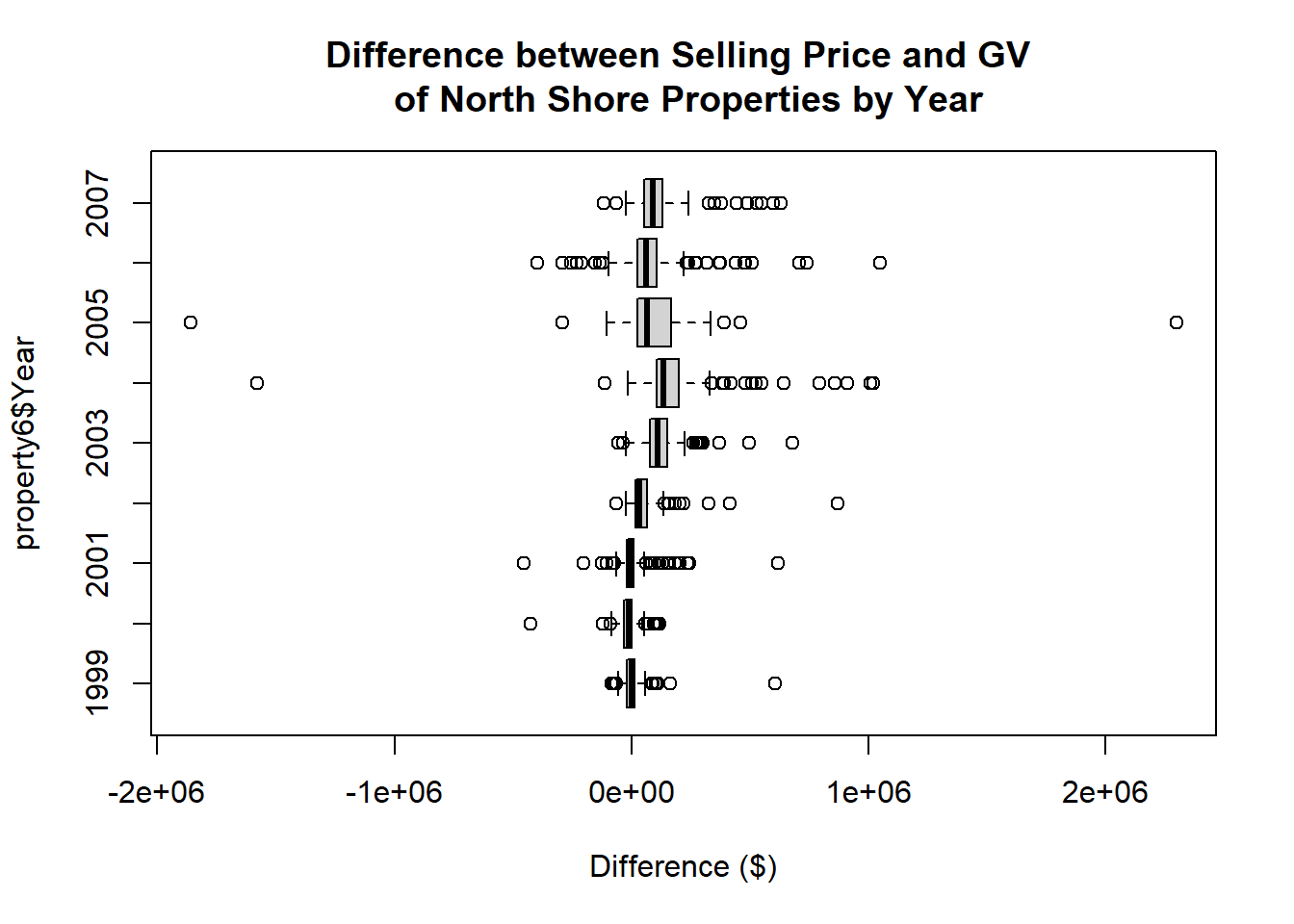

Previous Lesson

See Task 1a. (Section 3.0.2) in Cockles for interpretation of box plots.

6. Extension: All techniques

Extension

If you wish to practice the techniques shown in this lesson some more, there are 2 additional sets of North Shore property data available.

The first has 6437 entries from 2006 to December 2007.

Download North Shore 2007.xls

The second has 9281 entries from 2006 to December 2008.

Download North Shore 2008.xls